There are several instances when having a scroll bar linked to an Excel chart can come in handy – it’s a great way to make your chart dynamic and can really enhance the functionality of an Excel dashboard. On this page, we’ll describe how to add a scroll bar to your Excel chart – in Excel 2007. We’ll provide an example file, created using the steps, with the completed chart and scroll bar. This will allow you to check your result against ours or use the example in your own project.
How to Add a Scroll Bar in Excel
Scroll Bar Example Download
Download 53.50 KB 939 downloadsStep 1
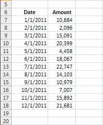
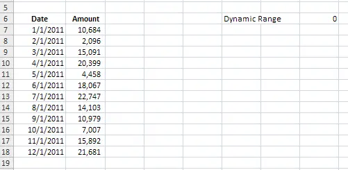
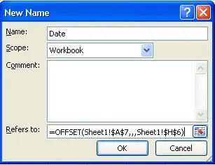
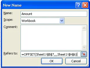
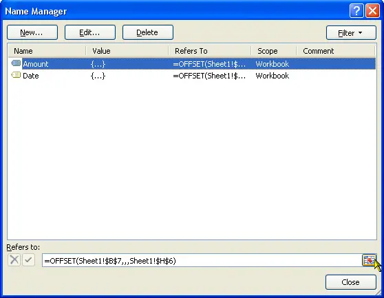
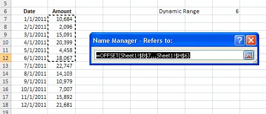
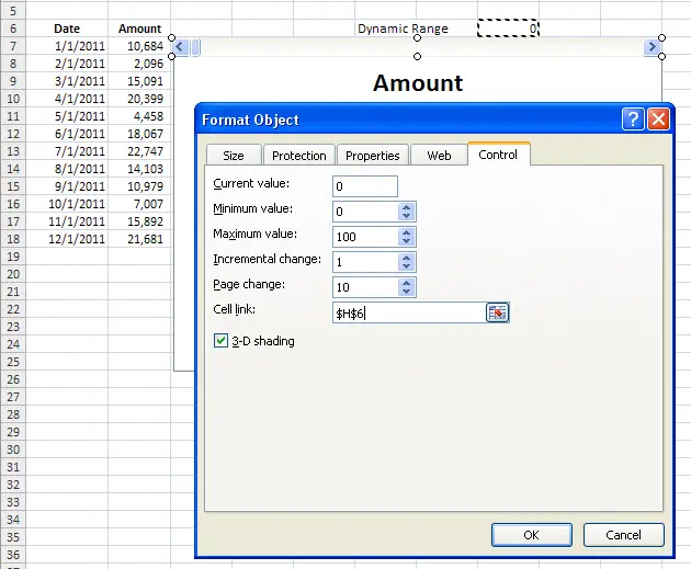
Next, determine where you want your dynamic range – this is the cell that is ultimately going to drive the data that’s reflected within your chart. Typically, I like to put this cell somewhere that will not show up when the data & chart are printed, and will not be deleted. If you simply want it hidden, you can always cut and paste it under your chart once the chart has been created. For this example we set ours up like this:
Step 3
Step 4
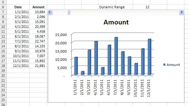
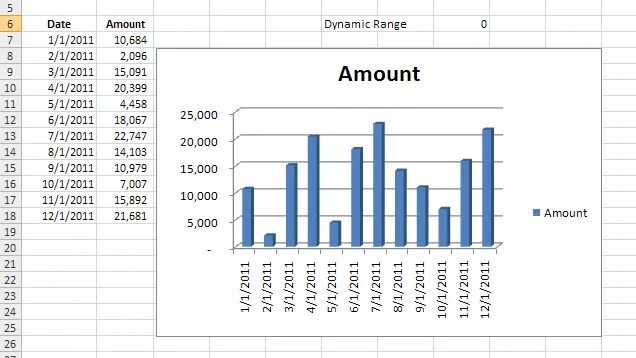
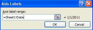
Here we’ll insert the chart. For this example, we’ve selected a 3-D bar chart. To add the chart, select cell A7 > select the ‘Insert’ ribbon > ‘Column’ > ‘3-D Column’. The following chart will be created.
Step 5
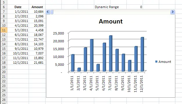
The last piece we need to include is the scroll bar. To do this, first enable your ‘Developer’ ribbon (Excel Orb > Excel Options > Popular > Check the box for ‘Show Developer tab). Under the ‘Developer’ ribbon choose Insert > Scroll Bar. Then, insert the scroll bar where you want it – we put it right over the chart.
Step 6
You’re Done!